Calculating Spin-Spin Coupling (J-Coupling) Constants
Background
Experimental NMR spectra contain a depth of information about each constituent atom in a structure and the interactions between atoms. While NMR shieldings pertain to a single atom in their surrounding medium (see: the Shieldings, NMR, and Magnetizabilities tutorials), the effective spin-spin interactions between different nuclei (J-couplings) also include effects of the electrons around them (this tutorial). In principle, it is possible to compute shieldings, magnetizabilities simultaneously in FHI-aims. However, very specific basis sets are necessary for accurate computation of J-couplings - in contrast, basis sets that are good for standard electronic structure calculations can lead to J-couplings that are wildly off from the converged result (see Laasner et al. 2024, as well as the broader literature on J-couplings). The reason is that much of the interesting response of the electrons to the presence of as nuclear spin arises at the nucleus and therefore, basis functions close to the nucleus must be included to capture this response.
Thus, J-couplings should only be computed with basis sets that are intended and tested for this computation.
The short answer is that the NAO-J-n basis sets or Jensen's Gaussian-based pcJ-n basis sets may both be used for J-coupling calculations (see below for details).
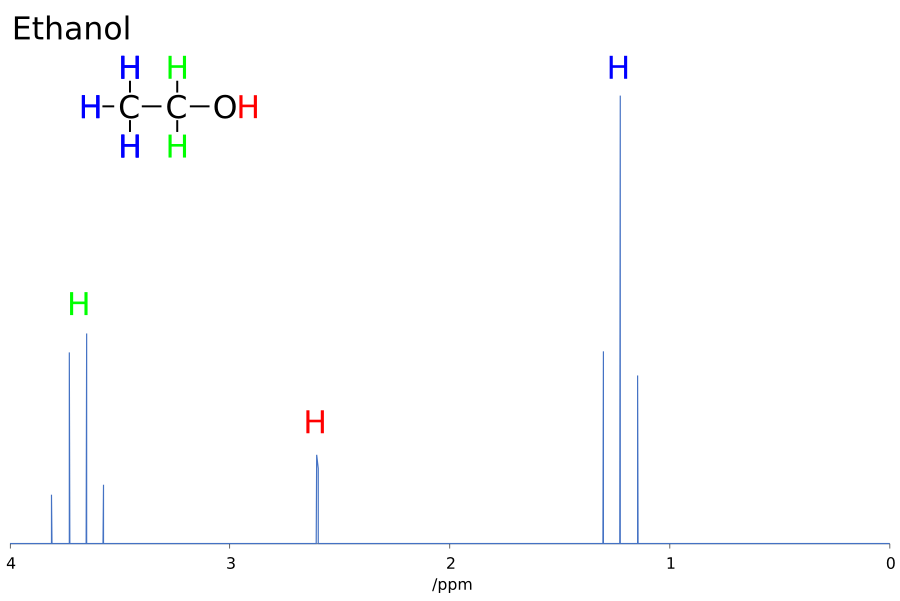
J-couplings, or spin-spin couplings, arise when two atoms with non-zero nuclear magnetic spin indirectly interact. In a NMR spectrum, the magnitude of the J-coupling appears as a frequency difference between the spins of each atom in a pair. This frequency is independent of the applied magnetic field and thus is always expressed in Hz. The sign of a J-coupling reveals whether the spins being parallel (negative J-coupling) or 180° from each other (positive J-coupling) is the lower energy state. In experimental NMR spectra, J-couplings are expressed as multiple clustered peaks around a feature (see Figure 1). These multiplicities can become complicated even for relatively simple molecules like ethanol but relay both the number of nuclei coupled to the atom of interest and the relative spin of these nuclei. The sensitivity of these couplings and their magnitude to the local chemical environment of a nuclei means that information both about bond distances and bond angles can be inferred from these J-couplings. The simulation of these couplings can help verify the link between the geometry and coupling.
Beyond the mere interpretation of NMR spectra, J-couplings are also generally responsible for the time evolution of coupled nuclear spins, e.g., enabling the coordinated transfer of spin polarization from one nucleus to another in techniques such as Signal Amplification By Reversible Exchange (SABRE, i.e. Pravdivtsev et al.)

Figure 1: Experimental 1H NMR Spectra for CH3CH2OH (Andel Früh, 2019)
Tutorial
Step 1: Setup
In this tutorial, we will calculate the J-Coupling constants for CH2O, one of the molecules that was part of a larger set of benchmarks in San Fabian et al..
This tutorial assumes basic knowledge of FHIaims calculations. If this is not the case, see: FHIaims.
San Fabian et al. did not, to our knowledge, publish their exact molecular geometries, but rather provided the method by which their geometries were optimized. In Laasner et al., we therefore optimized our own version of the geometry of CH2O, using the PBE0 hybrid density functional and FHI-aims' tight settings. The resulting, optimized geometry.in.next_step file looks as follows:
atom       0.93938451      0.00000000     -0.58605424 H
atom      -0.93938451      0.00000000     -0.58605424 H
atom       0.00000000      0.00000000      0.00000000 C
atom       0.00000000      0.00000000      1.19469036 O

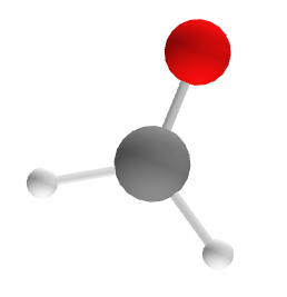
Figure 2: CH2O (Geometry optimized using the methodology of San Fabian et al.)
For the purposes of this tutorial, two other geometry optimizations were performed to compare both to this result from Laasner et al. and to compare to the reference values from San Fabian et al. PBE0 is a hybrid functional which mixes exact exchange from Hartree-Fock theory with ab initio or empirical exchange and correlation. This functional is relatively computationally expensive. PBE is a less expensive generalized gradient approximation (GGA) functional which is commonly used across DFT calculations. Thus, the structure of CH2O was also optimized at the level of PBE. In the original San Fabian work, no mention of relativistic correction is mentioned and the impact of such a correction is likely low due to the small atoms involved in CH2O. However, for other structure optimizations, relativistic corrections may be necessary so at the PBE level for the purposes of this tutorial, CH2O was optimized both including scalar relativistic effects and without any relativistic correction. As is standard for such computations, this structure was optimized using the following control.in file:
# control.in
xc              pbe
        vdw_correction_hirshfeld
relativistic    atomic_zora scalar
relax_geometry  bfgs 5e-3
spin            none

+ ['tight' FHIaims species defaults for H, C, and O]
In the non-relativistic case simply change the relativistic line to read relativistic none. These calculations should converge quickly (~3 seconds locally on my MacBook with an M1 processor). The resultant non-relativistic geometry.in.next_step file was computed as:
atom       0.94701660      0.00000000     -0.59254977 H
atom      -0.94701660      0.00000000     -0.59254977 H
atom       0.00000000     -0.00000000      0.00009919 C
atom      -0.00000000      0.00000000      1.20758223 O
The resultant relativistic geometry.in.next_step file was computed as:
atom       0.94708577     -0.00000000     -0.59263468 H
atom      -0.94708577     -0.00000000     -0.59263468 H
atom       0.00000000      0.00000000      0.00012682 C
atom      -0.00000000     -0.00000000      1.20772443 O
Step 2: J-coupling calculation
With energy optimized geometries, J-coupling values can now be computed. In order to request this calculation from FHI-aims, the following input geometry.in file may be used. Note the magnetic_response keyword in the geometry.in file after each atom which will be included in the J-coupling calculation (in this case both hydrogen atoms and the carbon atom). This geometry file corresponds to the non-relativistic PBE geometry, but equivalent geometry.in can be derived for both the relativistic PBE and non-relativistic PBE0 cases.
# geometry.in
atom       0.94701660      0.00000000     -0.59254977 H
magnetic_response
atom      -0.94701660      0.00000000     -0.59254977 H
magnetic_response
atom       0.00000000     -0.00000000      0.00009919 C
magnetic_response
atom      -0.00000000      0.00000000      1.20758223 O
In the control.in file, the magnetic_response j keyword indicates that J-couplings is the NMR parameter being computed in this calculation (as opposed to shieldings or magnetizabilities). VERY IMPORTANT is the choice of basis sets when computing J-couplings. Because J-couplings reflect the interaction between nuclei, accurate description of core electron states is far more important than in most DFT calculations. Thus, specialized basis sets must be used. For a further discussion of basis set choices for such calculations see Laasner et al. 2024 and refer to Figure 7. In this tutorial, we will compare each of the 'NAO-J-n' basis sets found in the species_defaults/NAO-J-n/ folder of the base FHIaims directory.
# control.in
xc                      pbe
spin                    none
relativistic            none
basis_threshold         0.0
magnetic_response       j

+ ['NAO-J-n' FHIaims species defaults for H, C, and O]
Note that relativistic none is set despite the geometry being optimized relativistically. Relativistic J-couplings can be computed in FHIaims, but non-relativistic values anecdotally match reference values more precisely. From this computation, J-coupling values can be found in the human-readable aims.out. In particular, the following section of aims.out contains the desired values (these results correspond to the 'NAO-J-5' species defaults):
    Total:
              2              3
    1   4.504095E+01   1.675012E+02      1
    2                  1.675012E+02      2
Reformatted, the computed J-couplings can be found in the following table:
| Atoms | Computed J-coupling |
|---|---|
| 1 (H) - 2 (H) | 45.04095 Hz |
| 1 (H) - 3 (C) | 167.5012 Hz |
| 2 (H) - 3 (C) | 167.5012 Hz |
The reference value of the C-H J-coupling from San Fabian et al. is 168.61 Hz. The similarly computed result for each geometry (PBE0, PBE relativistic, PBE non-relativistic) can be found in the following table. As can be seen, computed J-couplings from FHIaims can approximate reference values to extremely high accuracy.
| Geometry Optimization | NAO-J-2 | NAO-J-3 | NAO-J-4 | NAO-J-5 |
|---|---|---|---|---|
| PBE0 non-relativistic | 164.50 Hz | 166.54 Hz | 166.89 Hz | 165.18 Hz |
| PBE non-relativistic | 166.70 Hz | 168.82 Hz | 169.18 Hz | 167.52 Hz |
| PBE relativistic | 166.68 Hz | 168.80 Hz | 169.16 Hz | 167.50 Hz |
In addition, for each case, the following total run times were observed:
| Geometry Optimization | NAO-J-2 | NAO-J-3 | NAO-J-4 | NAO-J-5 |
|---|---|---|---|---|
| PBE0 non-relativistic | 17.168 s | 28.108 s | 51.270 s | 106.963 s |
| PBE non-relativistic | 17.214 s | 27.332 s | 49.878 s | 106.365 s |
| PBE relativistic | 17.135 s | 28.038 s | 50.958 s | 109.137 s |
Larger systems
The NAO-J basis sets are rather large (especially for well converged calculations) and they can therefore become badly conditioned for mid-sized molecules.
For other types of calculations, FHI-aims automatically detects this condition (so-called "ill-conditioned" basis set) and stops, asking the user to remedy the situation. If requested by the user (using the override_illconditioning keyword in control.in), the calculation could continue after removing components of the basis (more specifically, eigenvectors of the overlap matrix) with very small eigenvalues from the actuail basis set used in the production calculation. The default threshold for this reduction is basis_threshold 1d-5.
In J-coupling calculations, this is not the case.
In the current implementation of the J-coupling formalism, it is recommended to keep all basis functions in the basis set regardless, i.e., use keywords
override_illconditioning .true.
basis_threshold 0.d0
instead of reducing out components of the basis set.
For larger basis sets, an additional safeguard is to perform a convergence test (e.g., NAO-J2, NAO-J3, NAO-J4 in succession) and verify that the observed changes of the resulting J-couplings remain systematic and relatively small.